Differentiation of implicit functions
Suppose we have a quantity \(y\) defined implicitly as the solution of \(\begin{equation} f(x,y)=0 \end{equation}\)
For each value of \(x\), we take \(y(x)\) to be the solution of \((1)\). Now what is \(\frac{dy}{dx}\)?
Assuming that all the functions at play are sufficiently smooth, we can write \(\begin{align} 0 =& \frac{d}{dx} f\left(x,y(x)\right) \\ =& \frac{\partial f}{\partial x} + \left.\frac{\partial f}{\partial y}\right\rvert_{y(x)} \frac{dy}{dx} \end{align}\) which gives \(\begin{equation} \frac{dy}{dx} = - \frac{\frac{\partial f}{\partial x}}{\left.\frac{\partial f}{\partial y}\right\rvert_{y(x)}} \end{equation}\)
Example: the Belief Propagation equations.
For an Ising model on a regular graph of degree \(k\), the self-consistency equation for the cavity field \(u\) is \(\begin{equation} u = (k-1)\tanh^{-1}\left[\tanh(u)\tanh(J)\right] \end{equation}\) where \(J\) is the coupling strength.
For any value of \(J\), one computes \(u(J)\) as the fixed point of the above equation. Then, the magnetization is given by \(\begin{equation} m = \tanh\left(\beta \frac{k}{k-1}u(J)\right) \end{equation}\)
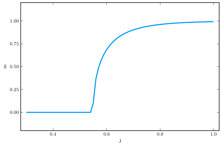
Here is what the \((m,J)\) plot looks like for \(k=3\)

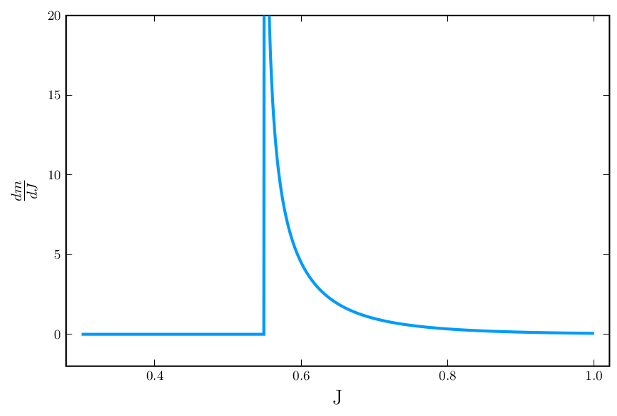
What is \(\frac{dm}{dJ}\)?
To make contact with the notation above, let’s define \(\begin{equation} f(J,u) = (k-1)\tanh^{-1}\left[\tanh(u)\tanh(J)\right] - u \end{equation}\) We are now able to compute the derivative of \(\frac{du}{dJ}\) using \((3)\) (as long as the denominator is nonzero).
Just a final chain rule \(\begin{align} \frac{dm}{dJ} =\left.\frac{dm}{du}\right\rvert_{u(J)}\frac{du}{dJ} \end{align}\) and we are done:

Not bad!
Here is the Julia code:
import ForwardDiff: derivative
using Plots, LaTeXStrings

pgfplotsx()
Plots.default(grid=:false, label="", msc=:auto, box=:on, labelfontsize=14)

k = 3
J = 1.0
β = 1.0

f(u, J) = (k-1)/β *atanh(tanh(β*u)*tanh(β*J))
g(u) = tanh(β*k/(k-1)*u)

function iterate_fixedpoint(f, init=1.0; maxiter=10^3, tol=1e-16)
    x = init
    err = Inf
    for _ in 1:maxiter
        xnew = f(x)
        abs(xnew) < tol && return 0.0
        err = abs((x-xnew)/x)
        err < tol && return x
        x = xnew
    end
    error("Fixed point iterations did not converge. err=$err")
end

Js = 0.3:1e-3:1.0
ms = zeros(length(Js))
dmdJs = zeros(length(Js))

for (i,J) in pairs(Js)
    ustar = iterate_fixedpoint(u->f(u,J), maxiter=10^5)
    dfdJ = derivative(J->f(ustar,J), J)
    dfdu = derivative(u->f(u,J), ustar)
    dudJ = dfdJ / (1 - dfdu)
    ms[i] = g(ustar)
    dmdJs[i] = dudJ * derivative(g, ustar)
end

pl = plot(Js, ms, xlabel="J", ylabel="m", ylims=(-0.2, 1.2))
pl2 = plot(Js, dmdJs, xlabel="J", ylabel=L"\frac{dm}{dJ}", ylims=(-2,20))